Dask for Machine Learning
Contents
Live Notebook
You can run this notebook in a live session 
Dask for Machine Learning
This is a high-level overview demonstrating some the components of Dask-ML. Visit the main Dask-ML documentation, see the dask tutorial notebook 08, or explore some of the other machine-learning examples.
[1]:
from dask.distributed import Client, progress
client = Client(processes=False, threads_per_worker=4,
                n_workers=1, memory_limit='2GB')
client
[1]:
Client
Client-12a6896d-0de0-11ed-9ba6-000d3a8f7959
| Connection method: Cluster object | Cluster type: distributed.LocalCluster |
| Dashboard: http://10.1.1.64:8787/status |
Cluster Info
LocalCluster
ced599b8
| Dashboard: http://10.1.1.64:8787/status | Workers: 1 |
| Total threads: 4 | Total memory: 1.86 GiB |
| Status: running | Using processes: False |
Scheduler Info
Scheduler
Scheduler-60443685-4058-48d1-ba10-996f80c21c06
| Comm: inproc://10.1.1.64/7078/1 | Workers: 1 |
| Dashboard: http://10.1.1.64:8787/status | Total threads: 4 |
| Started: Just now | Total memory: 1.86 GiB |
Workers
Worker: 0
| Comm: inproc://10.1.1.64/7078/4 | Total threads: 4 |
| Dashboard: http://10.1.1.64:42349/status | Memory: 1.86 GiB |
| Nanny: None | |
| Local directory: /home/runner/work/dask-examples/dask-examples/dask-worker-space/worker-0l66zwyz | |
Distributed Training

Scikit-learn uses joblib for single-machine parallelism. This lets you train most estimators (anything that accepts an n_jobs parameter) using all the cores of your laptop or workstation.
Alternatively, Scikit-Learn can use Dask for parallelism. This lets you train those estimators using all the cores of your cluster without significantly changing your code.
This is most useful for training large models on medium-sized datasets. You may have a large model when searching over many hyper-parameters, or when using an ensemble method with many individual estimators. For too small datasets, training times will typically be small enough that cluster-wide parallelism isn’t helpful. For too large datasets (larger than a single machine’s memory), the scikit-learn estimators may not be able to cope (see below).
Create Scikit-Learn Estimator
[2]:
from sklearn.datasets import make_classification
from sklearn.svm import SVC
from sklearn.model_selection import GridSearchCV
import pandas as pd
We’ll use scikit-learn to create a pair of small random arrays, one for the features X, and one for the target y.
[3]:
X, y = make_classification(n_samples=1000, random_state=0)
X[:5]
[3]:
array([[-1.06377997,  0.67640868,  1.06935647, -0.21758002,  0.46021477,
        -0.39916689, -0.07918751,  1.20938491, -0.78531472, -0.17218611,
        -1.08535744, -0.99311895,  0.30693511,  0.06405769, -1.0542328 ,
        -0.52749607, -0.0741832 , -0.35562842,  1.05721416, -0.90259159],
       [ 0.0708476 , -1.69528125,  2.44944917, -0.5304942 , -0.93296221,
         2.86520354,  2.43572851, -1.61850016,  1.30071691,  0.34840246,
         0.54493439,  0.22532411,  0.60556322, -0.19210097, -0.06802699,
         0.9716812 , -1.79204799,  0.01708348, -0.37566904, -0.62323644],
       [ 0.94028404, -0.49214582,  0.67795602, -0.22775445,  1.40175261,
         1.23165333, -0.77746425,  0.01561602,  1.33171299,  1.08477266,
        -0.97805157, -0.05012039,  0.94838552, -0.17342825, -0.47767184,
         0.76089649,  1.00115812, -0.06946407,  1.35904607, -1.18958963],
       [-0.29951677,  0.75988955,  0.18280267, -1.55023271,  0.33821802,
         0.36324148, -2.10052547, -0.4380675 , -0.16639343, -0.34083531,
         0.42435643,  1.17872434,  2.8314804 ,  0.14241375, -0.20281911,
         2.40571546,  0.31330473,  0.40435568, -0.28754632, -2.8478034 ],
       [-2.63062675,  0.23103376,  0.04246253,  0.47885055,  1.54674163,
         1.6379556 , -1.53207229, -0.73444479,  0.46585484,  0.4738362 ,
         0.98981401, -1.06119392, -0.88887952,  1.23840892, -0.57282854,
        -1.27533949,  1.0030065 , -0.47712843,  0.09853558,  0.52780407]])
We’ll fit a Support Vector Classifier, using grid search to find the best value of the \(C\) hyperparameter.
[4]:
param_grid = {"C": [0.001, 0.01, 0.1, 0.5, 1.0, 2.0, 5.0, 10.0],
              "kernel": ['rbf', 'poly', 'sigmoid'],
              "shrinking": [True, False]}

grid_search = GridSearchCV(SVC(gamma='auto', random_state=0, probability=True),
                           param_grid=param_grid,
                           return_train_score=False,
                           cv=3,
                           n_jobs=-1)
To fit that normally, we would call
grid_search.fit(X, y)
To fit it using the cluster, we just need to use a context manager provided by joblib.
[5]:
import joblib

with joblib.parallel_backend('dask'):
    grid_search.fit(X, y)
We fit 48 different models, one for each hyper-parameter combination in param_grid, distributed across the cluster. At this point, we have a regular scikit-learn model, which can be used for prediction, scoring, etc.
[6]:
pd.DataFrame(grid_search.cv_results_).head()
[6]:
| mean_fit_time | std_fit_time | mean_score_time | std_score_time | param_C | param_kernel | param_shrinking | params | split0_test_score | split1_test_score | split2_test_score | mean_test_score | std_test_score | rank_test_score | |
|---|---|---|---|---|---|---|---|---|---|---|---|---|---|---|
| 0 | 0.267177 | 0.011928 | 0.030591 | 0.006284 | 0.001 | rbf | True | {'C': 0.001, 'kernel': 'rbf', 'shrinking': True} | 0.502994 | 0.501502 | 0.501502 | 0.501999 | 0.000704 | 41 |
| 1 | 0.263738 | 0.005183 | 0.028903 | 0.005411 | 0.001 | rbf | False | {'C': 0.001, 'kernel': 'rbf', 'shrinking': False} | 0.502994 | 0.501502 | 0.501502 | 0.501999 | 0.000704 | 41 |
| 2 | 0.193400 | 0.005858 | 0.018773 | 0.003098 | 0.001 | poly | True | {'C': 0.001, 'kernel': 'poly', 'shrinking': True} | 0.502994 | 0.501502 | 0.501502 | 0.501999 | 0.000704 | 41 |
| 3 | 0.196229 | 0.006628 | 0.018826 | 0.002250 | 0.001 | poly | False | {'C': 0.001, 'kernel': 'poly', 'shrinking': Fa... | 0.502994 | 0.501502 | 0.501502 | 0.501999 | 0.000704 | 41 |
| 4 | 0.378106 | 0.006729 | 0.037400 | 0.002586 | 0.001 | sigmoid | True | {'C': 0.001, 'kernel': 'sigmoid', 'shrinking':... | 0.502994 | 0.501502 | 0.501502 | 0.501999 | 0.000704 | 41 |
[7]:
grid_search.predict(X)[:5]
[7]:
array([0, 1, 1, 1, 0])
[8]:
grid_search.score(X, y)
[8]:
0.983
For more on training scikit-learn models with distributed joblib, see the dask-ml documentation.
Training on Large Datasets
Most estimators in scikit-learn are designed to work on in-memory arrays. Training with larger datasets may require different algorithms.
All of the algorithms implemented in Dask-ML work well on larger than memory datasets, which you might store in a dask array or dataframe.
[9]:
%matplotlib inline
[10]:
import dask_ml.datasets
import dask_ml.cluster
import matplotlib.pyplot as plt
In this example, we’ll use dask_ml.datasets.make_blobs to generate some random dask arrays.
[11]:
X, y = dask_ml.datasets.make_blobs(n_samples=10000000,
                                   chunks=1000000,
                                   random_state=0,
                                   centers=3)
X = X.persist()
X
[11]:
|
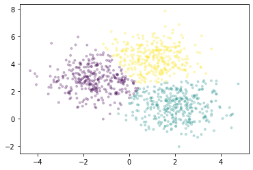
We’ll use the k-means implemented in Dask-ML to cluster the points. It uses the k-means|| (read: “k-means parallel”) initialization algorithm, which scales better than k-means++. All of the computation, both during and after initialization, can be done in parallel.
[12]:
km = dask_ml.cluster.KMeans(n_clusters=3, init_max_iter=2, oversampling_factor=10)
km.fit(X)
/usr/share/miniconda3/envs/dask-examples/lib/python3.9/site-packages/dask/base.py:1283: UserWarning: Running on a single-machine scheduler when a distributed client is active might lead to unexpected results.
  warnings.warn(
[12]:
KMeans(init_max_iter=2, n_clusters=3, oversampling_factor=10)
We’ll plot a sample of points, colored by the cluster each falls into.
[13]:
fig, ax = plt.subplots()
ax.scatter(X[::10000, 0], X[::10000, 1], marker='.', c=km.labels_[::10000],
           cmap='viridis', alpha=0.25);

For all the estimators implemented in Dask-ML, see the API documentation.