Singular Value Decomposition

Live Notebook

You can run this notebook in a live session or view it on Github.

Singular Value Decomposition¶

This notebook introduces the da.linalg.svd algorithms for the Singular Value Decomposition

Start Dask Client for Dashboard¶

Starting the Dask Client is optional. It will provide a dashboard which is useful to gain insight on the computation.

The link to the dashboard will become visible when you create the client below. We recommend having it open on one side of your screen while using your notebook on the other side. This can take some effort to arrange your windows, but seeing them both at the same is very useful when learning.

[1]:

from dask.distributed import Client, progress
client = Client(processes=False, threads_per_worker=4,
                n_workers=1, memory_limit='2GB')
client

[1]:

Client

Client-8ad1cc86-0de1-11ed-a4f6-000d3a8f7959

Connection method: Cluster object	Cluster type: distributed.LocalCluster
Dashboard: http://10.1.1.64:8787/status

Cluster Info

LocalCluster

9a88c089

Dashboard: http://10.1.1.64:8787/status	Workers: 1
Total threads: 4	Total memory: 1.86 GiB
Status: running	Using processes: False

Scheduler Info

Scheduler

Scheduler-ad8714da-ab0d-4c50-a4cb-ec68028ac54d

Comm: inproc://10.1.1.64/9462/1	Workers: 1
Dashboard: http://10.1.1.64:8787/status	Total threads: 4
Started: Just now	Total memory: 1.86 GiB

Workers

Worker: 0

Comm: inproc://10.1.1.64/9462/4	Total threads: 4
Dashboard: http://10.1.1.64:39957/status	Memory: 1.86 GiB
Nanny: None
Local directory: /home/runner/work/dask-examples/dask-examples/machine-learning/dask-worker-space/worker-we6_wppm

Compute SVD of Tall-and-Skinny Matrix¶

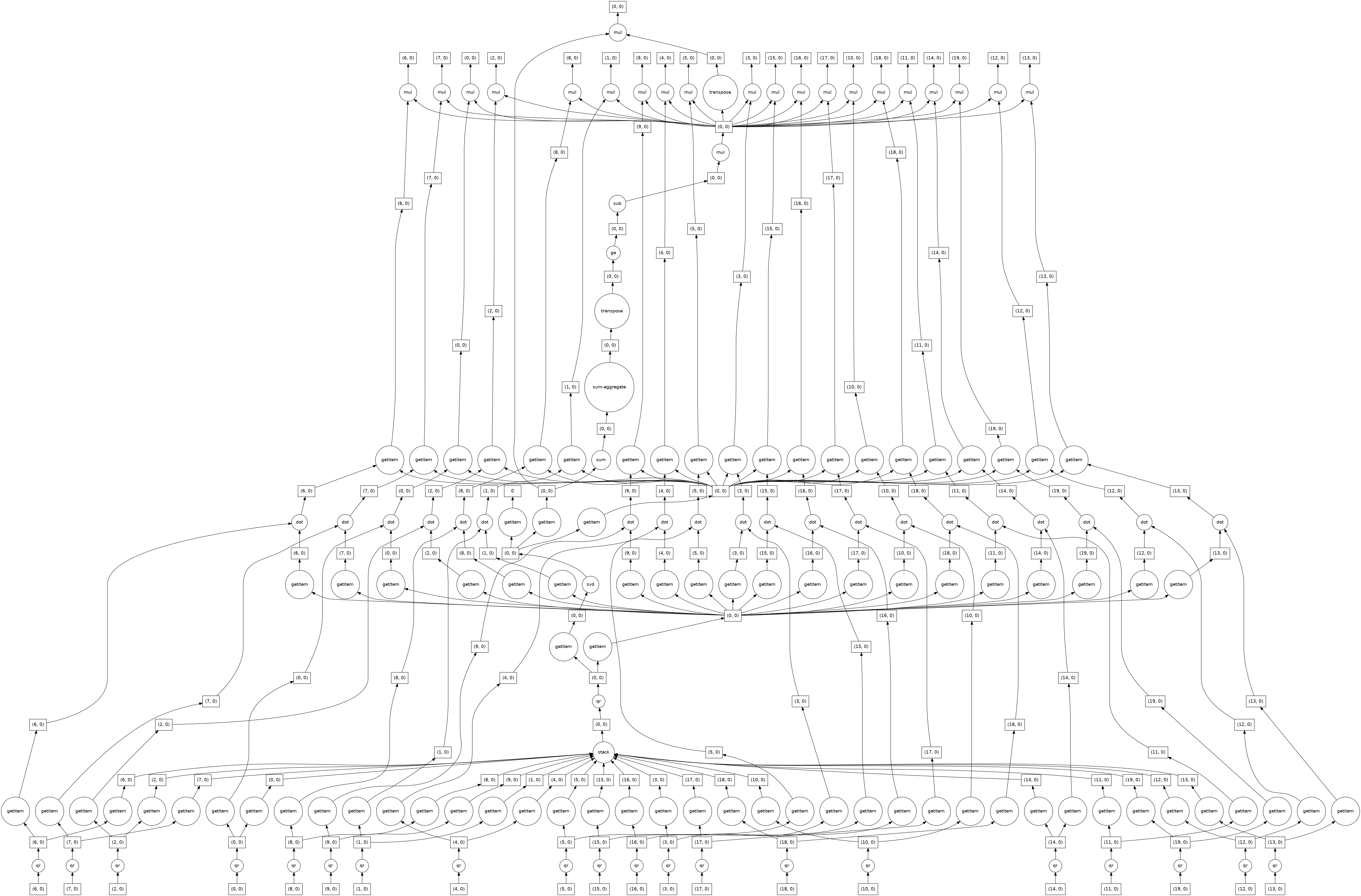
For many applications the provided matrix has many more rows than columns. In this case a specialized algorithm can be used.

[2]:

import dask.array as da

X = da.random.random((200000, 100), chunks=(10000, 100)).persist()

[3]:

import dask

u, s, v = da.linalg.svd(X)
dask.visualize(u, s, v)

[3]:

[4]:

v.compute()

[4]:

array([[ 0.09994831,  0.10007229,  0.09997617, ...,  0.09995264,
         0.09995591,  0.09984163],
       [ 0.05585195, -0.06184545, -0.04747733, ..., -0.06275421,
        -0.2061527 ,  0.18218227],
       [ 0.01277435,  0.00484692, -0.04387551, ...,  0.00444605,
         0.12143905, -0.06438531],
       ...,
       [ 0.02933106,  0.00834248,  0.0103009 , ..., -0.06069817,
         0.01291796,  0.12832988],
       [ 0.0901224 , -0.00492353, -0.00470015, ...,  0.14196305,
        -0.09734339, -0.05803211],
       [ 0.16619815,  0.14906927, -0.18081339, ..., -0.1346468 ,
         0.12524437,  0.01322112]])

Compute SVD of General Non-Skinny Matrix with Approximate algorithm¶

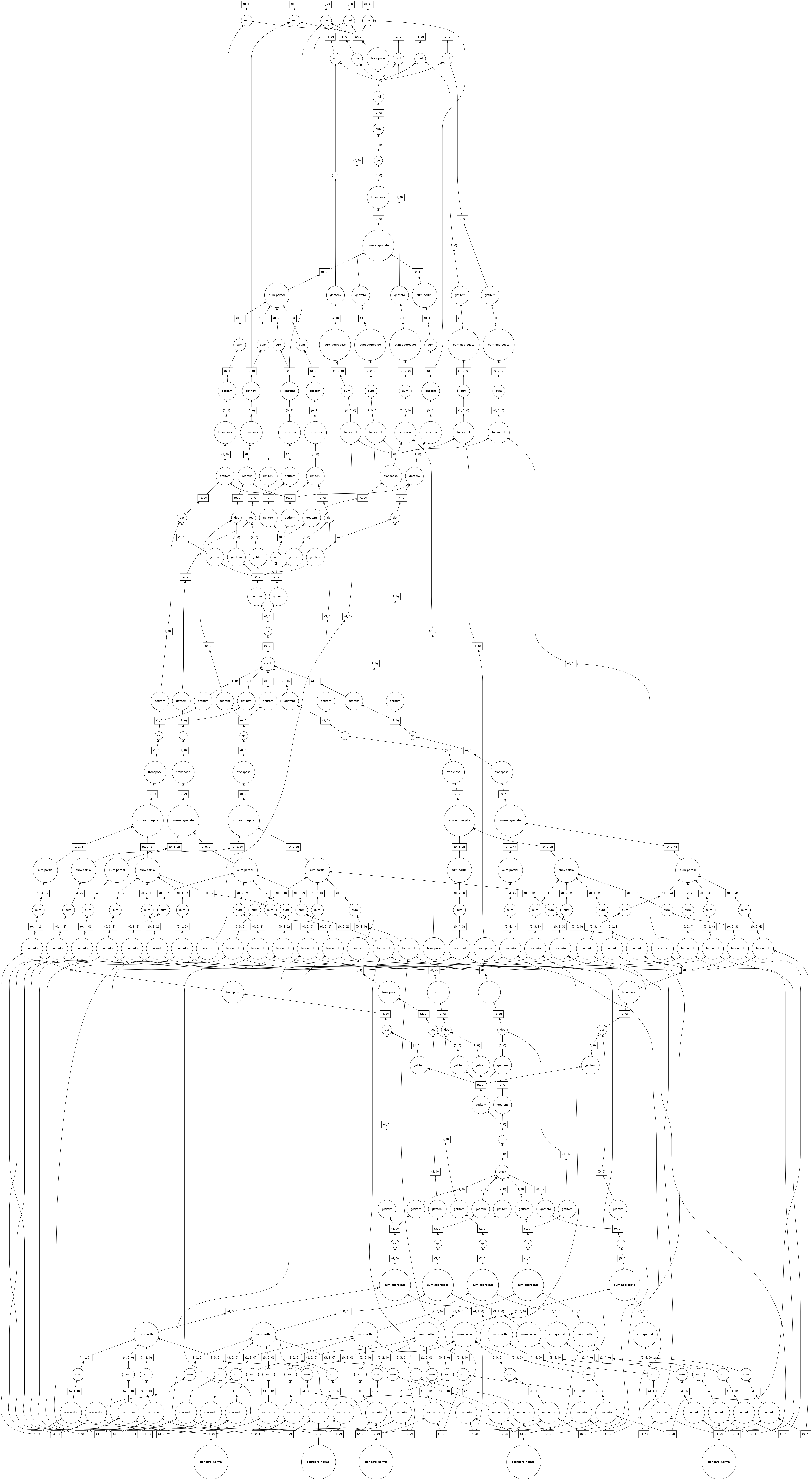
When there are also many chunks in columns then we use an approximate randomized algorithm to collect only a few of the singular values and vectors.

[5]:

import dask.array as da

X = da.random.random((10000, 10000), chunks=(2000, 2000)).persist()

[6]:

import dask

u, s, v = da.linalg.svd_compressed(X, k=5)
dask.visualize(u, s, v)

[6]:

[7]:

v.compute()

[7]:

array([[ 0.00997573,  0.01011564,  0.00997098, ...,  0.00998413,
         0.00994515,  0.0099736 ],
       [-0.00048293,  0.00247921, -0.00527027, ..., -0.00606932,
        -0.01272348,  0.00818248],
       [ 0.00145378, -0.00278148,  0.01078658, ..., -0.00428512,
        -0.00213905, -0.00738961],
       [-0.00984979, -0.00230993, -0.00277437, ...,  0.0056367 ,
        -0.00199535, -0.01409744],
       [-0.00210629, -0.00320545, -0.00190336, ...,  0.01871436,
        -0.01494592, -0.00274385]])

Generalized Linear Models

Analyze web-hosted JSON data

Dask Examples documentation