Dask DataFrames

Start Dask Client for Dashboard¶

Starting the Dask Client is optional. It will provide a dashboard which is useful to gain insight on the computation.

The link to the dashboard will become visible when you create the client below. We recommend having it open on one side of your screen while using your notebook on the other side. This can take some effort to arrange your windows, but seeing them both at the same is very useful when learning.

[1]:

from dask.distributed import Client

client = Client(n_workers=2, threads_per_worker=2, memory_limit="1GB")
client

[1]:

Client

Client-e0ebc4ca-0ddf-11ed-98b5-000d3a8f7959

Connection method: Cluster object	Cluster type: distributed.LocalCluster
Dashboard: http://127.0.0.1:8787/status

Cluster Info

LocalCluster

fb3316a9

Dashboard: http://127.0.0.1:8787/status	Workers: 2
Total threads: 4	Total memory: 1.86 GiB
Status: running	Using processes: True

Scheduler Info

Scheduler

Scheduler-44cb79c2-de9d-4ec5-8466-954570037d71

Comm: tcp://127.0.0.1:40039	Workers: 2
Dashboard: http://127.0.0.1:8787/status	Total threads: 4
Started: Just now	Total memory: 1.86 GiB

Workers

Worker: 0

Comm: tcp://127.0.0.1:38545	Total threads: 2
Dashboard: http://127.0.0.1:38797/status	Memory: 0.93 GiB
Nanny: tcp://127.0.0.1:41967
Local directory: /home/runner/work/dask-examples/dask-examples/dask-worker-space/worker-7ivifrfo

Worker: 1

Comm: tcp://127.0.0.1:36071	Total threads: 2
Dashboard: http://127.0.0.1:46269/status	Memory: 0.93 GiB
Nanny: tcp://127.0.0.1:37775
Local directory: /home/runner/work/dask-examples/dask-examples/dask-worker-space/worker-7ftt40fj

Create Random Dataframe¶

We create a random timeseries of data with the following attributes:

It stores a record for every second in the month of January of the year 2000
It splits that month by day, keeping each day as a partitioned dataframe
Along with a datetime index it has columns for names, ids, and numeric values

This is a small dataset of about 240 MB. Increase the number of days or reduce the time interval between data points to practice with a larger dataset by setting some of the `dask.datasets.timeseries() arguments <https://docs.dask.org/en/stable/api.html#dask.datasets.timeseries>`__.

[2]:

import dask

df = dask.datasets.timeseries()

Unlike Pandas, Dask DataFrames are lazy, meaning that data is only loaded when it is needed for a computation. No data is printed here, instead it is replaced by ellipses (...).

[3]:

df

[3]:

Dask DataFrame Structure:

	id	name	x	y
npartitions=30
2000-01-01	int64	object	float64	float64
2000-01-02	...	...	...	...
...	...	...	...	...
2000-01-30	...	...	...	...
2000-01-31	...	...	...	...

Dask Name: make-timeseries, 30 tasks

Nonetheless, the column names and dtypes are known.

[4]:

df.dtypes

[4]:

id        int64
name     object
x       float64
y       float64
dtype: object

Some operations will automatically display the data.

[5]:

# This sets some formatting parameters for displayed data.
import pandas as pd

pd.options.display.precision = 2
pd.options.display.max_rows = 10

[6]:

df.head(3)

[6]:

	id	name	x	y
timestamp
2000-01-01 00:00:00	999	Patricia	0.86	0.50
2000-01-01 00:00:01	974	Alice	-0.04	0.25
2000-01-01 00:00:02	984	Ursula	-0.05	-0.92

Use Standard Pandas Operations¶

Most common Pandas operations can be used in the same way on Dask dataframes. This example shows how to slice the data based on a mask condition and then determine the standard deviation of the data in the x column.

[7]:

df2 = df[df.y > 0]
df3 = df2.groupby("name").x.std()
df3

[7]:

Dask Series Structure:
npartitions=1
    float64
        ...
Name: x, dtype: float64
Dask Name: sqrt, 157 tasks

Notice that the data in df3 are still represented by ellipses. All of the operations in the previous cell are lazy operations. You can call .compute() when you want your result as a Pandas dataframe or series.

If you started Client() above then you can watch the status page during computation to see the progress.

[8]:

computed_df = df3.compute()
type(computed_df)

[8]:

pandas.core.series.Series

[9]:

computed_df

[9]:

name
Alice      0.58
Bob        0.58
Charlie    0.58
Dan        0.58
Edith      0.58
           ...
Victor     0.58
Wendy      0.58
Xavier     0.58
Yvonne     0.58
Zelda      0.58
Name: x, Length: 26, dtype: float64

Notice that the computed data are now shown in the output.

Another example calculation is to aggregate multiple columns, as shown below. Once again, the dashboard will show the progress of the computation.

[10]:

df4 = df.groupby("name").aggregate({"x": "sum", "y": "max"})
df4.compute()

[10]:

	x	y
name
Alice	172.30	1.0
Bob	54.79	1.0
Charlie	255.01	1.0
Dan	93.23	1.0
Edith	155.41	1.0
...	...	...
Victor	-303.80	1.0
Wendy	-20.97	1.0
Xavier	112.18	1.0
Yvonne	335.84	1.0
Zelda	205.43	1.0

26 rows × 2 columns

Dask dataframes can also be joined like Pandas dataframes. In this example we join the aggregated data in df4 with the original data in df. Since the index in df is the timeseries and df4 is indexed by names, we use left_on="name" and right_index=True to define the merge columns. We also set suffixes for any columns that are common between the two dataframes so that we can distinguish them.

Finally, since df4 is small, we also make sure that it is a single partition dataframe.

[11]:

df4 = df4.repartition(npartitions=1)
joined = df.merge(
    df4, left_on="name", right_index=True, suffixes=("_original", "_aggregated")
)
joined.head()

[11]:

	id	name	x_original	y_original	x_aggregated	y_aggregated
timestamp
2000-01-01 00:00:00	999	Patricia	0.86	0.50	-34.68	1.0
2000-01-01 00:00:03	988	Patricia	-0.57	-0.67	-34.68	1.0
2000-01-01 00:00:12	1038	Patricia	-0.48	0.35	-34.68	1.0
2000-01-01 00:01:16	964	Patricia	-0.25	0.13	-34.68	1.0
2000-01-01 00:01:33	1050	Patricia	-0.58	-0.38	-34.68	1.0

Persist data in memory¶

If you have the available RAM for your dataset then you can persist data in memory.

This allows future computations to be much faster.

[12]:

df = df.persist()

Time Series Operations¶

Because df has a datetime index, time-series operations work efficiently.

The first example below resamples the data at 1 hour intervals to reduce the total size of the dataframe. Then the mean of the x and y columns are taken.

[13]:

df[["x", "y"]].resample("1h").mean().head()

[13]:

	x	y
timestamp
2000-01-01 00:00:00	1.96e-03	1.43e-02
2000-01-01 01:00:00	5.23e-03	1.51e-02
2000-01-01 02:00:00	-9.91e-04	-9.25e-04
2000-01-01 03:00:00	-2.57e-03	-5.00e-03
2000-01-01 04:00:00	-5.71e-03	1.16e-02

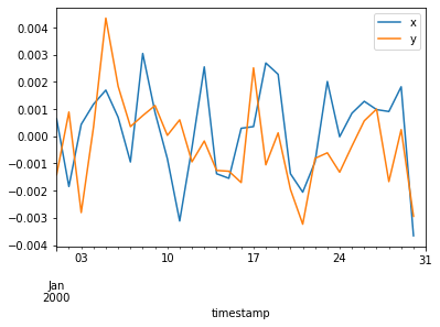
The next example resamples the data at 24 hour intervals and plots the mean values. Notice that plot() is called after compute() because plot() will not work until the data are computed.

[14]:

%matplotlib inline
df[['x', 'y']].resample('24h').mean().compute().plot();

This final example computes the rolling 24 hour mean of the data.

[15]:

df[["x", "y"]].rolling(window="24h").mean().head()

[15]:

	x	y
timestamp
2000-01-01 00:00:00	0.86	0.50
2000-01-01 00:00:01	0.41	0.38
2000-01-01 00:00:02	0.25	-0.05
2000-01-01 00:00:03	0.05	-0.21
2000-01-01 00:00:04	0.18	-0.18

Random access is cheap along the index, but must since the Dask dataframe is lazy, it must be computed to materialize the data.

[16]:

df.loc["2000-01-05"]

[16]:

Dask DataFrame Structure:

	id	name	x	y
npartitions=1
2000-01-05 00:00:00.000000000	int64	object	float64	float64
2000-01-05 23:59:59.999999999	...	...	...	...

Dask Name: loc, 31 tasks

[17]:

%time df.loc['2000-01-05'].compute()

CPU times: user 28.7 ms, sys: 7.62 ms, total: 36.3 ms
Wall time: 64.2 ms

[17]:

	id	name	x	y
timestamp
2000-01-05 00:00:00	1001	Hannah	0.85	-0.23
2000-01-05 00:00:01	1021	Charlie	-0.09	-0.42
2000-01-05 00:00:02	974	Zelda	0.70	-0.81
2000-01-05 00:00:03	1015	Sarah	0.35	-0.13
2000-01-05 00:00:04	989	Frank	-0.26	-0.96
...	...	...	...	...
2000-01-05 23:59:55	1023	Alice	0.68	0.21
2000-01-05 23:59:56	982	Alice	0.90	0.74
2000-01-05 23:59:57	941	Sarah	-0.49	-0.39
2000-01-05 23:59:58	1009	Kevin	0.89	-0.26
2000-01-05 23:59:59	1031	Hannah	0.80	0.53

86400 rows × 4 columns

Set Index¶

Data is sorted by the index column. This allows for faster access, joins, groupby-apply operations, and more. However sorting data can be costly to do in parallel, so setting the index is both important to do, but only infrequently. In the next few examples, we will group the data by the name column, so we will set that column as the index to improve efficiency.

[18]:

df5 = df.set_index("name")
df5

[18]:

Dask DataFrame Structure:

	id	x	y
npartitions=26
Alice	int64	float64	float64
Bob	...	...	...
...	...	...	...
Zelda	...	...	...
Zelda	...	...	...

Dask Name: sort_index, 954 tasks

Because resetting the index for this dataset is expensive and we can fit it in our available RAM, we persist the dataset to memory.

[19]:

df5 = df5.persist()
df5

[19]:

Dask DataFrame Structure:

	id	x	y
npartitions=26
Alice	int64	float64	float64
Bob	...	...	...
...	...	...	...
Zelda	...	...	...
Zelda	...	...	...

Dask Name: sort_index, 26 tasks

Dask now knows where all data lives, indexed by name. As a result operations like random access are cheap and efficient.

[20]:

%time df5.loc['Alice'].compute()

CPU times: user 360 ms, sys: 44.7 ms, total: 404 ms
Wall time: 2.35 s

[20]:

	id	x	y
name
Alice	974	-0.04	0.25
Alice	1001	0.44	0.55
Alice	1039	-0.38	0.88
Alice	974	-0.71	0.12
Alice	960	0.98	-0.21
...	...	...	...
Alice	994	0.56	0.90
Alice	999	0.03	-0.11
Alice	988	-0.49	-0.80
Alice	999	-0.35	-0.20
Alice	1079	-0.29	0.88

99801 rows × 3 columns

Groupby Apply with Scikit-Learn¶

Now that our data is sorted by name we can inexpensively do operations like random access on name, or groupby-apply with custom functions.

Here we train a different scikit-learn linear regression model on each name.

[21]:

from sklearn.linear_model import LinearRegression


def train(partition):
    if not len(partition):
        return
    est = LinearRegression()
    est.fit(partition[["x"]].values, partition.y.values)
    return est

The partition argument to train() will be one of the group instances from the DataFrameGroupBy. If there is no data in the partition, we don’t need to proceed. If there is data, we want to fit the linear regression model and return that as the value for this group.

Now working with df5, whose index is the names from df, we can group by the names column. This also happens to be the index, but that’s fine. Then we use .apply() to run train() on each group in the DataFrameGroupBy generated by .groupby().

The meta argument tells Dask how to create the DataFrame or Series that will hold the result of .apply(). In this case, train() returns a single value, so .apply() will create a Series. This means we need to tell Dask what the type of that single column should be and optionally give it a name.

The easiest way to specify a single column is with a tuple. The name of the column is the first element of the tuple. Since this is a series of linear regressions, we will name the column "LinearRegression". The second element of the tuple is the type of the return value of train. In this case, Pandas will store the result as a general object, which should be the type we pass.

[22]:

df6 = df5.groupby("name").apply(
    train, meta=("LinearRegression", object)
).compute()
df6

[22]:

name
Alice      LinearRegression()
Bob        LinearRegression()
Charlie    LinearRegression()
Dan        LinearRegression()
Edith      LinearRegression()
                  ...
Victor     LinearRegression()
Wendy      LinearRegression()
Xavier     LinearRegression()
Yvonne     LinearRegression()
Zelda      LinearRegression()
Name: LinearRegression, Length: 26, dtype: object

Dask Examples documentation

Contents

Dask DataFrames¶

Start Dask Client for Dashboard¶

Client

Cluster Info

LocalCluster

Scheduler Info

Scheduler

Workers

Worker: 0

Worker: 1

Create Random Dataframe¶

Use Standard Pandas Operations¶

Persist data in memory¶

Time Series Operations¶

Set Index¶

Groupby Apply with Scikit-Learn¶

Further Reading¶