Hyperparameter optimization with Dask
Contents
Live Notebook
You can run this notebook in a live session ![]() or view it on Github.
or view it on Github.
Hyperparameter optimization with Dask
Every machine learning model has some values that are specified before training begins. These values help adapt the model to the data but must be given before any training data is seen. For example, this might be penalty or C in Scikit-learn’s LogisiticRegression. These values that come before any training data and are called “hyperparameters”. Typical usage looks something like:
from sklearn.linear_model import LogisiticRegression
from sklearn.datasets import make_classification

X, y = make_classification()
est = LogisiticRegression(C=10, penalty="l2")
est.fit(X, y)
These hyperparameters influence the quality of the prediction. For example, if C is too small in the example above, the output of the estimator will not fit the data well.
Determining the values of these hyperparameters is difficult. In fact, Scikit-learn has an entire documentation page on finding the best values: https://scikit-learn.org/stable/modules/grid_search.html
Dask enables some new techniques and opportunities for hyperparameter optimization. One of these opportunities involves stopping training early to limit computation. Naturally, this requires some way to stop and restart training (partial_fit or warm_start in Scikit-learn parlance).
This is especially useful when the search is complex and has many search parameters. Good examples are most deep learning models, which has specialized algorithms for handling many data but have difficulty providing basic hyperparameters (e.g., “learning rate”, “momentum” or “weight decay”).
This notebook will walk through
setting up a realistic example
how to use
HyperbandSearchCV, includingunderstanding the input parameters to
HyperbandSearchCVrunning the hyperparameter optimization
how to access informantion from
HyperbandSearchCV
This notebook will specifically not show a performance comparison motivating HyperbandSearchCV use. HyperbandSearchCV finds high scores with minimal training; however, this is a tutorial on how to use it. All performance comparisons are relegated to section Learn more.
[1]:
%matplotlib inline
Setup Dask
[2]:
from distributed import Client
client = Client(processes=False, threads_per_worker=4,
                n_workers=1, memory_limit='2GB')
client
[2]:
Client
Client-6ab1bd16-0de1-11ed-a383-000d3a8f7959
| Connection method: Cluster object | Cluster type: distributed.LocalCluster |
| Dashboard: http://10.1.1.64:8787/status |
Cluster Info
LocalCluster
3d7b2964
| Dashboard: http://10.1.1.64:8787/status | Workers: 1 |
| Total threads: 4 | Total memory: 1.86 GiB |
| Status: running | Using processes: False |
Scheduler Info
Scheduler
Scheduler-c1bf35f0-8caf-4476-9919-060006f58f79
| Comm: inproc://10.1.1.64/9091/1 | Workers: 1 |
| Dashboard: http://10.1.1.64:8787/status | Total threads: 4 |
| Started: Just now | Total memory: 1.86 GiB |
Workers
Worker: 0
| Comm: inproc://10.1.1.64/9091/4 | Total threads: 4 |
| Dashboard: http://10.1.1.64:37053/status | Memory: 1.86 GiB |
| Nanny: None | |
| Local directory: /home/runner/work/dask-examples/dask-examples/machine-learning/dask-worker-space/worker-uj3a5b08 | |
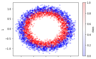
Create Data
[3]:
from sklearn.datasets import make_circles
import numpy as np
import pandas as pd

X, y = make_circles(n_samples=30_000, random_state=0, noise=0.09)

pd.DataFrame({0: X[:, 0], 1: X[:, 1], "class": y}).sample(4_000).plot.scatter(
    x=0, y=1, alpha=0.2, c="class", cmap="bwr"
);
Add random dimensions
[4]:
from sklearn.utils import check_random_state

rng = check_random_state(42)
random_feats = rng.uniform(-1, 1, size=(X.shape[0], 4))
X = np.hstack((X, random_feats))
X.shape
[4]:
(30000, 6)
Split and scale data
[5]:
from sklearn.model_selection import train_test_split
X_train, X_test, y_train, y_test = train_test_split(X, y, test_size=5_000, random_state=42)
[6]:
from sklearn.preprocessing import StandardScaler
from sklearn.model_selection import train_test_split
scaler = StandardScaler().fit(X_train)

X_train = scaler.transform(X_train)
X_test = scaler.transform(X_test)
[7]:
from dask.utils import format_bytes

for name, X in [("train", X_train), ("test", X_test)]:
    print("dataset =", name)
    print("shape =", X.shape)
    print("bytes =", format_bytes(X.nbytes))
    print("-" * 20)
dataset = train
shape = (25000, 6)
bytes = 1.14 MiB
--------------------
dataset = test
shape = (5000, 6)
bytes = 234.38 kiB
--------------------
Now we have our train and test sets.
Create model and search space
Let’s use Scikit-learn’s MLPClassifier as our model (for convenience). Let’s use this model with 24 neurons and tune some of the other basic hyperparameters.
[8]:
import numpy as np
from sklearn.neural_network import MLPClassifier

model = MLPClassifier()
Deep learning libraries can be used as well. In particular, PyTorch’s Scikit-Learn wrapper Skorch works well with HyperbandSearchCV.
[9]:
params = {
    "hidden_layer_sizes": [
        (24, ),
        (12, 12),
        (6, 6, 6, 6),
        (4, 4, 4, 4, 4, 4),
        (12, 6, 3, 3),
    ],
    "activation": ["relu", "logistic", "tanh"],
    "alpha": np.logspace(-6, -3, num=1000),  # cnts
    "batch_size": [16, 32, 64, 128, 256, 512],
}
Hyperparameter optimization
HyperbandSearchCV is Dask-ML’s meta-estimator to find the best hyperparameters. It can be used as an alternative to RandomizedSearchCV to find similar hyper-parameters in less time by not wasting time on hyper-parameters that are not promising. Specifically, it is almost guaranteed that it will find high performing models with minimal training.
This section will focus on
Understanding the input parameters to
HyperbandSearchCVUsing
HyperbandSearchCVto find the best hyperparametersSeeing other use cases of
HyperbandSearchCV
[10]:
from dask_ml.model_selection import HyperbandSearchCV
Determining input parameters
A rule-of-thumb to determine HyperbandSearchCV’s input parameters requires knowing:
the number of examples the longest trained model will see
the number of hyperparameters to evaluate
Let’s write down what these should be for this example:
[11]:
# For quick response
n_examples = 4 * len(X_train)
n_params = 8

# In practice, HyperbandSearchCV is most useful for longer searches
# n_examples = 15 * len(X_train)
# n_params = 15
In this, models that are trained the longest will see n_examples examples. This is how much data is required, normally set be the problem difficulty. Simple problems may only need 10 passes through the dataset; more complex problems may need 100 passes through the dataset.
There will be n_params parameters sampled so n_params models will be evaluated. Models with low scores will be terminated before they see n_examples examples. This helps perserve computation.
How can we use these values to determine the inputs for HyperbandSearchCV?
[12]:
max_iter = n_params  # number of times partial_fit will be called
chunks = n_examples // n_params  # number of examples each call sees

max_iter, chunks
[12]:
(8, 12500)
This means that the longest trained estimator will see about n_examples examples (specifically n_params * (n_examples // n_params).
Applying input parameters
Let’s create a Dask array with this chunk size:
[13]:
import dask.array as da
X_train2 = da.from_array(X_train, chunks=chunks)
y_train2 = da.from_array(y_train, chunks=chunks)
X_train2
[13]:
|
Each partial_fit call will receive one chunk.
That means the number of exmaples in each chunk should be (about) the same, and n_examples and n_params should be chosen to make that happen. (e.g., with 100 examples, shoot for chunks with (33, 33, 34) examples not (48, 48, 4) examples).
Now let’s use max_iter to create our HyperbandSearchCV object:
[14]:
search = HyperbandSearchCV(
    model,
    params,
    max_iter=max_iter,
    patience=True,
)
How much computation will be performed?
It isn’t clear how to determine how much computation is done from max_iter and chunks. Luckily, HyperbandSearchCV has a metadata attribute to determine this beforehand:
[15]:
search.metadata["partial_fit_calls"]
[15]:
26
This shows how many partial_fit calls will be performed in the computation. metadata also includes information on the number of models created.
So far, all that’s been done is getting the search ready for computation (and seeing how much computation will be performed). So far, all the computation has been quick and easy.
Performing the computation
Now, let’s do the model selection search and find the best hyperparameters. This is the real core of this notebook. This computation will be take place on all the hardware Dask has available.
[16]:
%%time
search.fit(X_train2, y_train2, classes=[0, 1, 2, 3])
/usr/share/miniconda3/envs/dask-examples/lib/python3.9/site-packages/dask_ml/model_selection/_incremental.py:641: VisibleDeprecationWarning: Creating an ndarray from ragged nested sequences (which is a list-or-tuple of lists-or-tuples-or ndarrays with different lengths or shapes) is deprecated. If you meant to do this, you must specify 'dtype=object' when creating the ndarray.
  cv_results = {k: np.array(v) for k, v in cv_results.items()}
/usr/share/miniconda3/envs/dask-examples/lib/python3.9/site-packages/dask_ml/model_selection/_hyperband.py:455: VisibleDeprecationWarning: Creating an ndarray from ragged nested sequences (which is a list-or-tuple of lists-or-tuples-or ndarrays with different lengths or shapes) is deprecated. If you meant to do this, you must specify 'dtype=object' when creating the ndarray.
  cv_results = {k: np.array(v) for k, v in cv_results.items()}
CPU times: user 3.54 s, sys: 661 ms, total: 4.2 s
Wall time: 3.42 s
[16]:
HyperbandSearchCV(estimator=MLPClassifier(), max_iter=8,
                  parameters={'activation': ['relu', 'logistic', 'tanh'],
                              'alpha': array([1.00000000e-06, 1.00693863e-06, 1.01392541e-06, 1.02096066e-06,
       1.02804473e-06, 1.03517796e-06, 1.04236067e-06, 1.04959323e-06,
       1.05687597e-06, 1.06420924e-06, 1.07159340e-06, 1.07902879e-06,
       1.08651577e-06, 1.09405471e-06, 1.10164595e-06, 1.1...
       9.01477631e-04, 9.07732653e-04, 9.14031075e-04, 9.20373200e-04,
       9.26759330e-04, 9.33189772e-04, 9.39664831e-04, 9.46184819e-04,
       9.52750047e-04, 9.59360829e-04, 9.66017480e-04, 9.72720319e-04,
       9.79469667e-04, 9.86265846e-04, 9.93109181e-04, 1.00000000e-03]),
                              'batch_size': [16, 32, 64, 128, 256, 512],
                              'hidden_layer_sizes': [(24,), (12, 12),
                                                     (6, 6, 6, 6),
                                                     (4, 4, 4, 4, 4, 4),
                                                     (12, 6, 3, 3)]},
                  patience=True)
The dashboard will be active while this is running. It will show which workers are running partial_fit and score calls. This takes about 10 seconds.
Integration
HyperbandSearchCV follows the Scikit-learn API and mirrors Scikit-learn’s RandomizedSearchCV. This means that it “just works”. All the Scikit-learn attributes and methods are available:
[17]:
search.best_score_
[17]:
0.8122
[18]:
search.best_estimator_
[18]:
MLPClassifier(alpha=1.0642092440647246e-05, batch_size=32,
              hidden_layer_sizes=(12, 12))
[19]:
cv_results = pd.DataFrame(search.cv_results_)
cv_results.head()
[19]:
| param_alpha | mean_partial_fit_time | std_partial_fit_time | bracket | mean_score_time | test_score | param_batch_size | std_score_time | param_hidden_layer_sizes | model_id | rank_test_score | param_activation | partial_fit_calls | params | |
|---|---|---|---|---|---|---|---|---|---|---|---|---|---|---|
| 0 | 0.000953 | 0.394128 | 0.026214 | 1 | 0.016661 | 0.7246 | 64 | 0.007632 | (24,) | bracket=1-0 | 1 | relu | 6 | {'hidden_layer_sizes': (24,), 'batch_size': 64... |
| 1 | 0.000159 | 0.785529 | 0.025667 | 1 | 0.020612 | 0.0000 | 256 | 0.003827 | (4, 4, 4, 4, 4, 4) | bracket=1-1 | 3 | logistic | 2 | {'hidden_layer_sizes': (4, 4, 4, 4, 4, 4), 'ba... |
| 2 | 0.000004 | 0.575372 | 0.035262 | 1 | 0.021490 | 0.5682 | 32 | 0.010454 | (24,) | bracket=1-2 | 2 | relu | 2 | {'hidden_layer_sizes': (24,), 'batch_size': 32... |
| 3 | 0.000003 | 0.455648 | 0.001261 | 0 | 0.021098 | 0.0000 | 512 | 0.001401 | (4, 4, 4, 4, 4, 4) | bracket=0-0 | 2 | relu | 3 | {'hidden_layer_sizes': (4, 4, 4, 4, 4, 4), 'ba... |
| 4 | 0.000011 | 0.266258 | 0.047284 | 0 | 0.008451 | 0.8122 | 32 | 0.004509 | (12, 12) | bracket=0-1 | 1 | relu | 8 | {'hidden_layer_sizes': (12, 12), 'batch_size':... |
[20]:
search.score(X_test, y_test)
[20]:
0.8036
[21]:
search.predict(X_test)
[21]:
|
[22]:
search.predict(X_test).compute()
[22]:
array([1, 0, 1, ..., 1, 0, 0])
It also has some other attributes.
[23]:
hist = pd.DataFrame(search.history_)
hist.head()
[23]:
| model_id | params | partial_fit_calls | partial_fit_time | score | score_time | elapsed_wall_time | bracket | |
|---|---|---|---|---|---|---|---|---|
| 0 | bracket=0-0 | {'hidden_layer_sizes': (4, 4, 4, 4, 4, 4), 'ba... | 1 | 0.454387 | 0.0000 | 0.022499 | 0.839712 | 0 |
| 1 | bracket=0-1 | {'hidden_layer_sizes': (12, 12), 'batch_size':... | 1 | 0.322257 | 0.5270 | 0.014936 | 0.839714 | 0 |
| 2 | bracket=1-0 | {'hidden_layer_sizes': (24,), 'batch_size': 64... | 1 | 0.431628 | 0.5138 | 0.007477 | 0.851272 | 1 |
| 3 | bracket=1-1 | {'hidden_layer_sizes': (4, 4, 4, 4, 4, 4), 'ba... | 1 | 0.811195 | 0.0000 | 0.024439 | 0.851274 | 1 |
| 4 | bracket=1-2 | {'hidden_layer_sizes': (24,), 'batch_size': 32... | 1 | 0.610634 | 0.5018 | 0.011036 | 0.851274 | 1 |
This illustrates the history after every partial_fit call. There’s also an attributed model_history_ that records the history for each model (it’s a reorganization of history_).
Learn more
This notebook covered basic usage HyperbandSearchCV. The following documentation and resources might be useful to learn more about HyperbandSearchCV, including some of the finer use cases:
A talk introducing
HyperbandSearchCVto the SciPy 2019 audience and the corresponding paper
Performance comparisons can be found in the SciPy 2019 talk/paper.