Image Processing
Contents
Live Notebook
You can run this notebook in a live session ![]() or view it on Github.
or view it on Github.
Image Processing
Welcome to the quickstart guide for dask-image.
Setting up your environment
Install Extra Dependencies
We first install the library scikit-image for easier access to the example image data there.
If you are running this notebook on your own computer and not in the mybinder environment, you’ll additionally need to ensure your Python environment contains: * dask * dask-image * python-graphviz * scikit-image * matplotlib * numpy
You can refer to the full list of dependencies used for the dask-examples repository, available in the `binder/environment.yml file here <https://github.com/dask/dask-examples/blob/main/binder/environment.yml>`__ (note that the nomkl package is not available for Windows users): https://github.com/dask/dask-examples/blob/main/binder/environment.yml
Importing dask-image
When you import dask-image, be sure to use an underscore instead of a dash between the two words.
[1]:
import dask_image.imread
import dask_image.ndfilters
import dask_image.ndmeasure
import dask.array as da
We’ll also use matplotlib to display image results in this notebook.
[2]:
import matplotlib.pyplot as plt
%matplotlib inline
Getting the example data
We’ll use some example image data from the scikit-image library in this tutorial. These images are very small, but will allow us to demonstrate the functionality of dask-image.
Let’s download and save a public domain image of the astronaut Eileen Collins to a temporary directory. This image was originally downloaded from the NASA Great Images database https://flic.kr/p/r9qvLn, but we’ll access it with scikit-image’s data.astronaut() method.
[3]:
!mkdir temp
[4]:
import os
from skimage import data, io

output_filename = os.path.join('temp', 'astronaut.png')
io.imsave(output_filename, data.astronaut())
Really large datasets often can’t fit all of the data into a single file, so we’ll chop this image into four parts and save the image tiles to a second temporary directory. This will give you a better idea of how you can use dask-image on a real dataset.
[5]:
!mkdir temp-tiles
[6]:
io.imsave(os.path.join('temp-tiles', 'image-00.png'), data.astronaut()[:256, :256, :])  # top left
io.imsave(os.path.join('temp-tiles', 'image-01.png'), data.astronaut()[:256, 256:, :])  # top right
io.imsave(os.path.join('temp-tiles', 'image-10.png'), data.astronaut()[256:, :256, :])  # bottom left
io.imsave(os.path.join('temp-tiles', 'image-11.png'), data.astronaut()[256:, 256:, :])  # bottom right
Now we have some data saved, let’s practise reading in files with dask-image and processing our images.
Reading in image data
Reading a single image
Let’s load a public domain image of the astronaut Eileen Collins with dask-image imread(). This image was originally downloaded from the NASA Great Images database https://flic.kr/p/r9qvLn.
[7]:
import os
filename = os.path.join('temp', 'astronaut.png')
print(filename)
temp/astronaut.png
[8]:
astronaut = dask_image.imread.imread(filename)
print(astronaut)
plt.imshow(astronaut[0, ...])  # display the first (and only) frame of the image
dask.array<_map_read_frame, shape=(1, 512, 512, 3), dtype=uint8, chunksize=(1, 512, 512, 3), chunktype=numpy.ndarray>
[8]:
<matplotlib.image.AxesImage at 0x7f0fb95fff40>
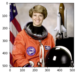
This has created a dask array with shape=(1, 512, 512, 3). This means it contains one image frame with 512 rows, 512 columns, and 3 color channels.
Since the image is relatively small, it fits entirely within one dask-image chunk, with chunksize=(1, 512, 512, 3).
Reading multiple images
In many cases, you may have multiple images stored on disk, for example: image_00.png, image_01.png, … image_NN.png. These can be read into a dask array as multiple image frames.
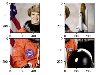
Here we have the astronaut image split into four non-overlapping tiles: * image_00.png = top left image (index 0,0) * image_01.png = top right image (index 0,1) * image_10.png = bottom left image (index 1,0) * image_11.png = bottom right image (index 1,1)
This filename pattern can be matched with regex: image-*.png
[9]:
!ls temp-tiles
image-00.png image-01.png image-10.png image-11.png
[10]:
import os
filename_pattern = os.path.join('temp-tiles', 'image-*.png')
tiled_astronaut_images = dask_image.imread.imread(filename_pattern)
print(tiled_astronaut_images)
dask.array<_map_read_frame, shape=(4, 256, 256, 3), dtype=uint8, chunksize=(1, 256, 256, 3), chunktype=numpy.ndarray>
This has created a dask array with shape=(4, 256, 256, 3). This means it contains four image frames; each with 256 rows, 256 columns, and 3 color channels.
There are four chunks in this particular case. Each image frame here is a separate chunk with chunksize=(1, 256, 256, 3).
[11]:
fig, ax = plt.subplots(nrows=2, ncols=2)
ax[0,0].imshow(tiled_astronaut_images[0])
ax[0,1].imshow(tiled_astronaut_images[1])
ax[1,0].imshow(tiled_astronaut_images[2])
ax[1,1].imshow(tiled_astronaut_images[3])
plt.show()
Applying your own custom function to images
Next you’ll want to do some image processing, and apply a function to your images.
We’ll use a very simple example: converting an RGB image to grayscale. But you can also use this method to apply arbittrary functions to dask images. To convert our image to grayscale, we’ll use the equation to calculate luminance (reference pdf)“:
Y = 0.2125 R + 0.7154 G + 0.0721 B
We’ll write the function for this equation as follows:
[12]:
def grayscale(rgb):
    result = ((rgb[..., 0] * 0.2125) +
              (rgb[..., 1] * 0.7154) +
              (rgb[..., 2] * 0.0721))
    return result
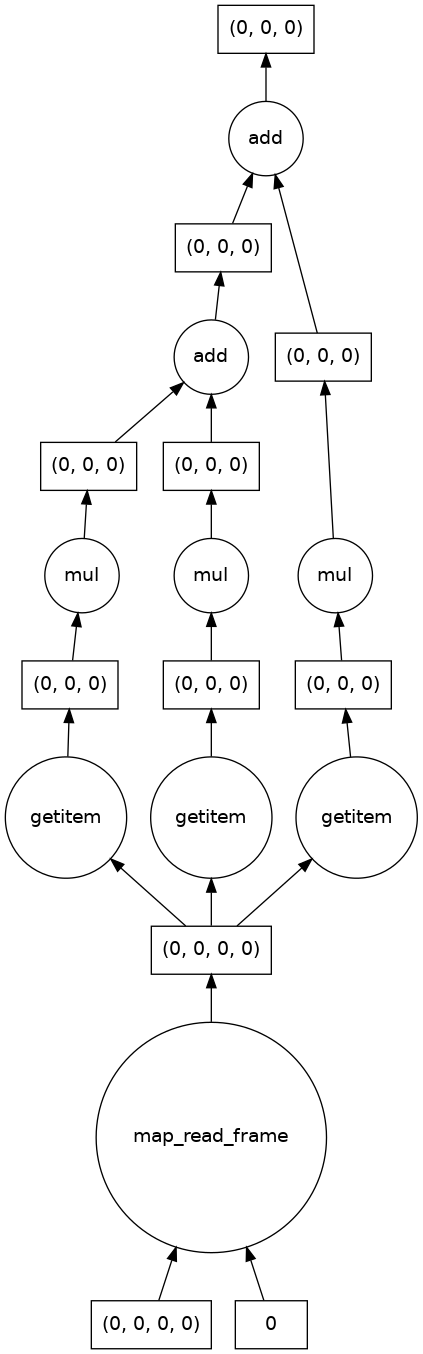
Let’s apply this function to the astronaut image we read in as a single file and visualize the computation graph.
(Visualizing the computation graph isn’t necessary most of the time but it’s helpful to know what dask is doing under the hood, and it can also be very useful for debugging problems.)
[13]:
single_image_result = grayscale(astronaut)
print(single_image_result)
single_image_result.visualize()
dask.array<add, shape=(1, 512, 512), dtype=float64, chunksize=(1, 512, 512), chunktype=numpy.ndarray>
[13]:
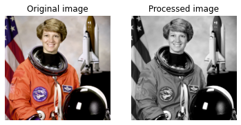
We also see that there are no longer three color channels in the shape of the result, and that the output image is as expected.
[14]:
print("Original image dimensions: ", astronaut.shape)
print("Processed image dimensions:", single_image_result.shape)

fig, (ax0, ax1) = plt.subplots(nrows=1, ncols=2)
ax0.imshow(astronaut[0, ...])            # display the first (and only) frame of the image
ax1.imshow(single_image_result[0, ...], cmap='gray')  # display the first (and only) frame of the image

# Subplot headings
ax0.set_title('Original image')
ax1.set_title('Processed image')

# Don't display axes
ax0.axis('off')
ax1.axis('off')

# Display images
plt.show(fig)
Original image dimensions:  (1, 512, 512, 3)
Processed image dimensions: (1, 512, 512)
Embarrassingly parallel problems
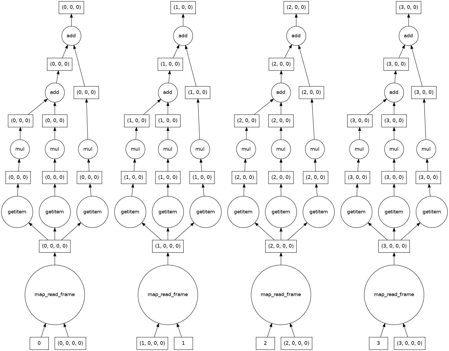
The syntax is identical to apply a function to multiple images or dask chunks. This is an example of an embarrassingly parallel problem, and we see that dask automatically creates a computation graph for each chunk.
[15]:
result = grayscale(tiled_astronaut_images)
print(result)
result.visualize()
dask.array<add, shape=(4, 256, 256), dtype=float64, chunksize=(1, 256, 256), chunktype=numpy.ndarray>
[15]:
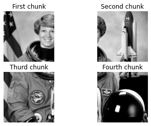
Let’s take a look at the results.
[16]:
fig, ((ax0, ax1), (ax2, ax3)) = plt.subplots(nrows=2, ncols=2)
ax0.imshow(result[0, ...], cmap='gray')
ax1.imshow(result[1, ...], cmap='gray')
ax2.imshow(result[2, ...], cmap='gray')
ax3.imshow(result[3, ...], cmap='gray')

# Subplot headings
ax0.set_title('First chunk')
ax1.set_title('Second chunk')
ax2.set_title('Thurd chunk')
ax3.set_title('Fourth chunk')

# Don't display axes
ax0.axis('off')
ax1.axis('off')
ax2.axis('off')
ax3.axis('off')

# Display images
plt.show(fig)
Joining partial images together
OK, Things are looking pretty good! But how can we join these image chunks together?
So far, we haven’t needed any information from neighboring pixels to do our calculations. But there are lots of functions (like those in dask-image ndfilters) that do need this for accurate results. You could end up with unwanted edge effects if you don’t tell dask how your images should be joined.
Dask has several ways to join chunks together: Stack, Concatenate, and Block.
Block is very versatile, so we’ll use that in this next example. You simply pass in a list (or list of lists) to tell dask the spatial relationship between image chunks.
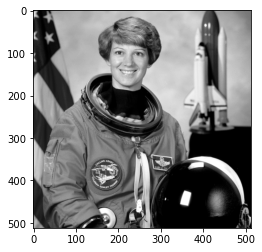
[17]:
data = [[result[0, ...], result[1, ...]],
        [result[2, ...], result[3, ...]]]
combined_image = da.block(data)
print(combined_image.shape)
plt.imshow(combined_image, cmap='gray')
(512, 512)
[17]:
<matplotlib.image.AxesImage at 0x7f0fb8187e80>
A segmentation analysis pipeline
We’ll walk through a simple image segmentation and analysis pipeline with three steps: 1. Filtering 1. Segmenting 1. Analyzing
Filtering
Most analysis pipelines require some degree of image preprocessing. dask-image has a number of inbuilt filters available via dask-image ndfilters
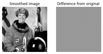
Commonly a guassian filter may used to smooth the image before segmentation. This causes some loss of sharpness in the image, but can improve segmentation quality for methods that rely on image thresholding.
[18]:
smoothed_image = dask_image.ndfilters.gaussian_filter(combined_image, sigma=[1, 1])
We see a small amount of blur in the smoothed image.
[19]:
fig, (ax0, ax1) = plt.subplots(nrows=1, ncols=2)
ax0.imshow(smoothed_image, cmap='gray')
ax1.imshow(smoothed_image - combined_image, cmap='gray')

# Subplot headings
ax0.set_title('Smoothed image')
ax1.set_title('Difference from original')

# Don't display axes
ax0.axis('off')
ax1.axis('off')

# Display images
plt.show(fig)
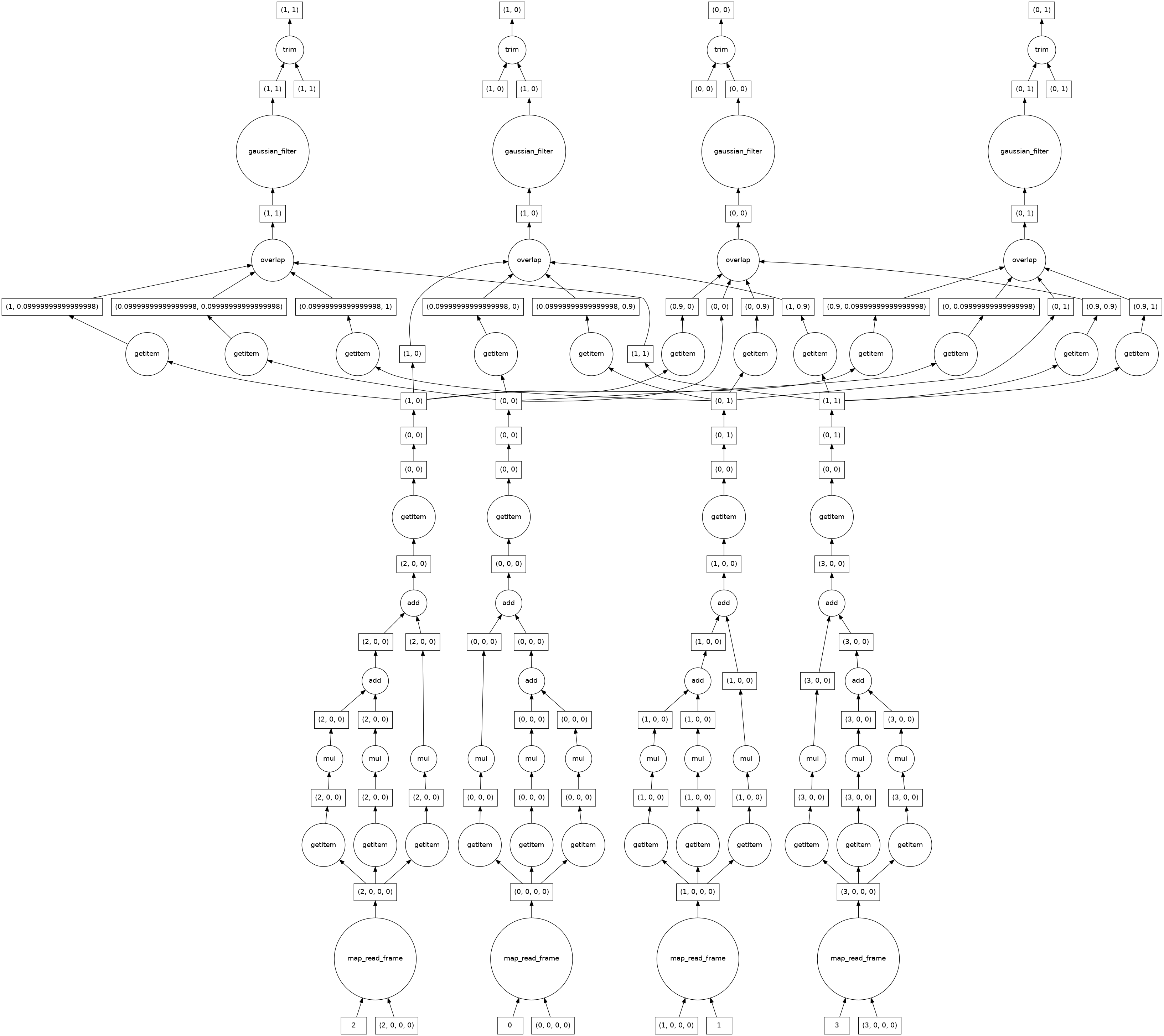
Since the gaussian filter uses information from neighbouring pixels, the computational graph looks more complicated than the ones we looked at earlier. This is no longer embarrassingly parallel. Where possible dask keeps the computations for each of the four image chunks separate, but must combine information from different chunks near the edges.
[20]:
smoothed_image.visualize()
[20]:
Segmenting
After the image preprocessing, we segment regions of interest from the data. We’ll use a simple arbitrary threshold as the cutoff, at 75% of the maximum intensity of the smoothed image.
[21]:
threshold_value = 0.75 * da.max(smoothed_image).compute()
print(threshold_value)
190.5550614819934
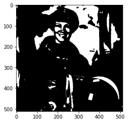
[22]:
threshold_image = smoothed_image > threshold_value
plt.imshow(threshold_image, cmap='gray')
[22]:
<matplotlib.image.AxesImage at 0x7f0fb82f9d00>
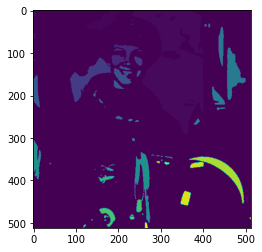
Next, we label each region of connected pixels above the threshold value. For this we use the label function from dask-image ndmeasure. This will return both the label image, and the number of labels.
[23]:
label_image, num_labels = dask_image.ndmeasure.label(threshold_image)
[24]:
print("Number of labels:", int(num_labels))
plt.imshow(label_image, cmap='viridis')
Number of labels: 78
[24]:
<matplotlib.image.AxesImage at 0x7f0fb801c760>
Analyzing
There are a number of inbuilt functions in dask-image ndmeasure useful for quantitative analysis.
We’ll use the dask_image.ndmeasure.mean() and dask_image.ndmeasure.standard_deviation() functions, and apply them to each label region with dask_image.ndmeasure.labeled_comprehension().
[25]:
index = list(range(int(num_labels)))  # Note that we're including the background label=0 here, too.
out_dtype = float  # The data type we want to use for our results.
default = None     # The value to return if an element of index does not exist in the label image.
mean_values = dask_image.ndmeasure.labeled_comprehension(combined_image, label_image, index, dask_image.ndmeasure.mean, out_dtype, default, pass_positions=False)
print(mean_values.compute())
[ 90.87492186 194.69185981 207.76964212 215.16959146 196.92609412
 206.50032105 217.0948     211.0477766  205.68146    208.61031956
 212.43803803 201.39967857 210.291275   198.3529809  201.21037636
 214.13041176 200.9344975  201.85547778 194.46485714 202.60302231
 205.20927983 203.72510602 205.94798756 205.88514047 207.33728
 216.13305227 206.7058     211.6957     211.75921279 224.71301613
 249.08085    215.87763779 198.27655577 213.67658483 205.65810758
 197.46586082 202.35786579 199.16034783 216.27194848 200.69137594
 220.99142573 207.66165    234.37771667 224.00188182 229.2705
 232.9163     187.1873     236.16183793 223.7469     187.813475
 227.4778     244.17155    225.49225806 239.4951     218.7795
 242.99015132 232.4975218  201.98308947 230.57158889 212.82135217
 242.21528571 241.32428889 228.722932   220.1454     239.55
 246.5        241.53348    236.28736    244.84466624 242.09528
 203.37236667 209.34061875 213.76621346 247.53468249 252.488826
 208.5659     197.72356    203.13211   ]
Since we’re including label 0 in our index, it’s not surprising that the first mean value is so much lower than the others - it’s the background region below our cutoff threshold for segmentation.
Let’s also calculate the standard deviation of the pixel values in our greyscale image.
[26]:
stdev_values = dask_image.ndmeasure.labeled_comprehension(combined_image, label_image, index, dask_image.ndmeasure.standard_deviation, out_dtype, default, pass_positions=False)
Finally, let’s load our analysis results into a pandas table and then save it as a csv file.
[27]:
import pandas as pd

df = pd.DataFrame()
df['label'] = index
df['mean'] = mean_values.compute()
df['standard_deviation'] = stdev_values.compute()

df.head()
[27]:
| label | mean | standard_deviation | |
|---|---|---|---|
| 0 | 0 | 90.874922 | 65.452828 |
| 1 | 1 | 194.691860 | 2.921235 |
| 2 | 2 | 207.769642 | 11.411058 |
| 3 | 3 | 215.169591 | 9.193374 |
| 4 | 4 | 196.926094 | 5.215053 |
[28]:
df.to_csv('example_analysis_results.csv')
print('Saved example_analysis_results.csv')
Saved example_analysis_results.csv
Next steps
I hope this guide has helped you to get started with dask-image.
Documentation
You can read more about dask-image in the dask-image documentation and API reference. Documentation for dask is here.
The dask-examples repository has a number of other example notebooks: https://github.com/dask/dask-examples
Scaling up with dask distributed
If you want to send dask jobs to a computing cluster for distributed processing, you should take a look at dask distributed. There is also a quickstart guide available.
Saving image data with zarr
In some cases it may be necessary to save large data after image processing, zarr is a python library that you may find useful.
Cleaning up temporary directories and files
You recall we saved some example data to the directories temp/ and temp-tiles/. To delete the contents, run the following command:
[29]:
!rm -r temp
[30]:
!rm -r temp-tiles